| Visit DIX: German-Spanish-German dictionary | diccionario Alemán-Castellano-Alemán | Spanisch-Deutsch-Spanisch Wörterbuch |
In this chapter the data structure of a tensor is studied. First a mathematical insight of tensor data is given. Some measurements related to tensor characteristics are presented, followed by different ways of applying transformations on tensors. Finally the visualization of a tensor is discussed.
A scalar is a quantity whose specification (in any coordinate system)
requires just one number. A tensor of order ![]() on the other hand is an
object that requires
on the other hand is an
object that requires ![]() numbers in any given coordinate
system. With this definition, scalars and vectors are special cases of
a tensor. Scalars are tensors of order 0 with
numbers in any given coordinate
system. With this definition, scalars and vectors are special cases of
a tensor. Scalars are tensors of order 0 with ![]() components,
and vectors are tensors of order 1 with
components,
and vectors are tensors of order 1 with ![]() components. The
diffusion tensors are general tensors of order 2 with
components. The
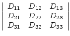
diffusion tensors are general tensors of order 2 with ![]() components. The components of a second order tensor are often written
as a
components. The components of a second order tensor are often written
as a ![]() matrix, as will be done here. Moreover the diffusion
tensor is a symmetric second order tensor so that the matrix is of the
form
matrix, as will be done here. Moreover the diffusion
tensor is a symmetric second order tensor so that the matrix is of the
form
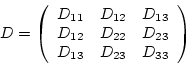 |
(4.1) |
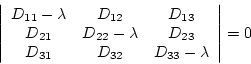
A tensor can be reduced to principal axes (eigenvalue and eigenvector decomposition) if the equation
| (4.2) |
| (4.3) |
Let
![]() be the eigenvalues of
the symmetric tensor
be the eigenvalues of
the symmetric tensor ![]() and let
and let
![]() be the normalized
eigenvector corresponding to
be the normalized
eigenvector corresponding to ![]() .
As the diffusion tensor is symmetric the eigenvalues
.
As the diffusion tensor is symmetric the eigenvalues ![]() will always be real.
Moreover the corresponding eigenvectors are perpendicular.
will always be real.
Moreover the corresponding eigenvectors are perpendicular.
The values ![]() can be found by solving the characteristic equation
can be found by solving the characteristic equation
 |
(4.4) |
Therefore the quantities
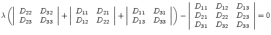
The inverse transformation from an eigensystem to a tensor is given by
| (4.9) |
| (4.10) |
| (4.11) |
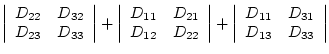
A general diffusion tensor ![]() will be a combination of these
cases. Expanding the diffusion tensor using these base cases gives:
will be a combination of these
cases. Expanding the diffusion tensor using these base cases gives:
| (4.12) |
| (4.16) |
![\fbox{\includegraphics[width = 0.8\textwidth]{images/randomfieldb.ps}}](img147.gif)
|
![\fbox{\includegraphics[width = 0.8\textwidth]{images/randomfieldbg3.ps}}](img148.gif)
|
![[*]](crossref.gif) , when the displacement
of a tensorfield is discussed.
, when the displacement
of a tensorfield is discussed.
Unlike scalar data the tensor is a three dimensional structure at each voxel position. Therefore simple grayscale images are not suitable for the representation of tensor data. Some ways of displaying tensor fields are presented and discussed here.
The tensor can be represented as an ellipsoid where the main axes lengths correspond to the eigenvalues and their direction to the respective eigenvectors. This method of display has already been used to illustrate the tensor characteristics in the previous section.
However, when displaying tensors as ellipsoids, there is no difference between an edge-on, flat ellipsoid, and an oblong one, or between a face-on, flat ellipsoid, and a sphere. By assigning a specular intensity and power to the ellipsoids, the reflection of the light source gives an insight of the third dimension of the ellipsoid. This allows a distinction between the ambiguous cases mentioned. Also the field can be rotated in all three dimensions so that the ellipsoids can be inspectioned from any direction.
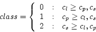
In the implementation, the tensors are classified into three different classes depending on their shape, and color-encoded according to the class they belong to. The tensors are assigned to a class depending on how close to a line, plane or sphere they are:
 |
(4.18) |
Figure 4.7 illustrates this displaying technique, where class 0 tensors are displayed in blue, class 1 tensors in yellow and class 2 tensors in yellow with the transparency set to 0.4.
![\fbox{\includegraphics[width = 0.8\textwidth]{images/westinslice11_5.ps}}](img152.gif)
|
The representation of a tensorfield in ellipsoids is certainly limited in size, since the overall information provided is too large for a visual inspection. Therefore two dimensional representations of the tensors are useful when observing larger objects.
One way of visualizing the tensors as two-dimensional objects it to
use blue headless arrows that represent the in-plane components of
![]() [17]. The out-of-plane components of
[17]. The out-of-plane components of
![]() are shown in colors ranging from green through
yellow to red, with red indicating the highest value for this
component. Figure 4.8 shows the example slice using
this visualization technique.
are shown in colors ranging from green through
yellow to red, with red indicating the highest value for this
component. Figure 4.8 shows the example slice using
this visualization technique.
Figure 4.9 shows another way of color encoding the
eigenvector corresponding to the largest eigenvalue. Here the
components of the first eigenvector
![]() ,
,
![]() and
and
![]() are multiplied by
the length of the eigenvalue
are multiplied by
the length of the eigenvalue ![]() . The red, green and blue
(RGB) values for the color at a position
. The red, green and blue
(RGB) values for the color at a position ![]() are then set to
are then set to
| (4.19) |
The disadvantage of this form of visualization is that fibertracts change color when changing direction, even though these color changes will be smooth. Nevertheless, it is a useful visualization to get an impression of the quality and the content of the data set.
![\includegraphics[width = 0.8\textwidth]{images/matlabtensor2.eps}](img165.gif)
|
![\includegraphics[width = 0.8\textwidth]{images/mycolor.ps}](img166.gif)
|
Finally the different measurements presented in Section 4.2 can be represented as grayscale images. Figure 4.10, 4.11 and 4.12 show this measurements for the same subject.
![\includegraphics[width = 0.8\textwidth]{images/closeline.ps}](img167.gif)
|
![\includegraphics[width = 0.8\textwidth]{images/closeplane.ps}](img168.gif)
|
The program main allows the display of any tensorfield which has been
preprocessed as described in Chapter 5. The
displaying of tensor data sets with ellipsoids is a very computation
intensive process. It is therefore recommended that in displaying an
image that one begins with a very small data window to see if the
result is presented in a
reasonable time.
![\fbox{\includegraphics[width = 0.8\textwidth]{images/randomfield.ps}}](img145.gif)
![\fbox{\includegraphics[width = 0.8\textwidth]{images/randomfieldg5.ps}}](img146.gif)
![\fbox{\includegraphics[width = 0.9\textwidth]{images/tensortransformation1.ps}}](img149.gif)
![\fbox{\includegraphics[width = 0.9\textwidth]{images/tensortransformation2.ps}}](img150.gif)
![\includegraphics[width = 0.4\textwidth]{images/closesphere.ps}](img169.gif)